
By Dylan Blechner, Zak Koeppel, Will Friedeman, Cameron Johnson
Introduction
What do the four teams playing on conference championship weekend (Chiefs, Patriots, Rams, and Saints) have in common? They are the top four scoring offenses in the National Football League. The league is shifting toward needing an elite offense in order to win games and advance in the playoffs. Having an above average quarterback is usually important, but if you can design plays to get receivers open, almost any league average quarterback can succeed with an optimally-constructed offense. This made identifying the best receiver-route combinations an intriguing topic for us to investigate. This data should be used by NFL coaches to design plays and game plan against opponents each week. More specifically, if you know your next opponent employs a lot of nickel defense, you can adjust your game plan with plays which have been proven most successful against nickel defense. In this paper, we analyze routes to identify the best route combinations a team can use.
Route Clustering
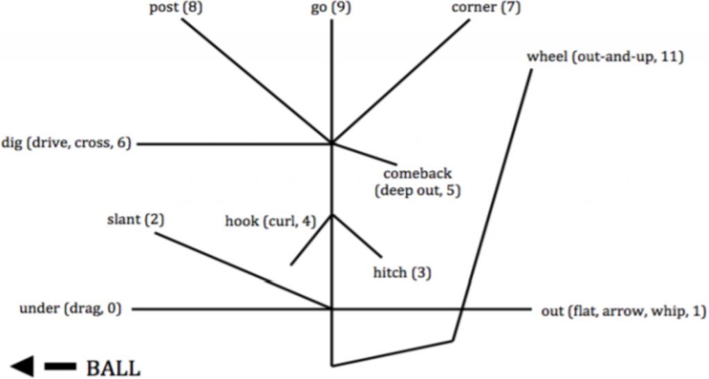
When trying to identify the best receiver-route combinations in the NFL, we felt it necessary to use the data provided to better classify each of the routes run during last year’s season. When doing research on the subject to find the best way to classify NFL routes, we came upon a paper from the MIT Sloan Sports Analytics Conference in 2017 that dealt with the same issue. The paper titled American Football Route Identification Using Supervised Machine Learning by Jeremy Hochstedler and Paul T. Gagnon used RFID tracking technology to best categorize receiver routes. The study took a look at the Indianapolis Colts in particular and used data similar to the Next Gen Stats data provided in this competition. Trained coaches assisting in the study classified each route in association with a simple route tree shown below.
The study attempted to use machine learning techniques to create an accurate model which predicts the correct classification of receiver routes. Hochstetler and Gagnon’s model included five factors to predict a receiver’s route: stem length, branch angle, average speed, final x-coordinate, and final y-coordinate. Using these factors, the study used a 1:1 train-to-test ratio to predict routes using the following machine learning classification methods: Naive Bayes, k-Nearest Neighbors, Random Forest, Logistic Regression, and Support Vector Machines (SVM). We felt this paper replicated our final goal of classifying receiver routes and our access of Next Gen Stats tracking data could improve their model and results. Because we did not have any help from a football coach telling us what each route was supposed to be, we felt clustering the routes by the five factors previously mentioned would be the best way to group them. We clustered the data using the two main unsupervised machine learning techniques: K Means Clustering and Hierarchical Clustering. After evaluating the results, we found that hierarchical clustering gave us more reliable and intuitive clusters that mimicked an NFL route tree.
Five Factors
The first two factors we had to calculate were the stem length and branch angle. The Sloan Analytics study suggested that all routes have three main points: a stem, pivot point, and branch. For example, in the slant route shown below, the original two to three-yard straight segment would be considered the stem, the position where the direction changes would be the pivot point, and the end segment would be the branch.
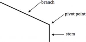
By using a segmented or piecewise regression in R, the route can be separated into two pieces and then the stem length and branch angle can be measured. The problem with running a segmented regression using the “segmented” package in R is that the pivot point must be known to create the stem and branch. To find the pivot point, we used the same technique referenced in Hochstetler and Gagnon, which was to minimize the Euclidean distance (linear distance between two points) between the first and last points in the route. To find the first point in the route, we used the x and y-coordinates when the ball was snapped. This point was given a location of (0,0) and all other points were relative to this one. We then found the Euclidean distance between the first point and every other point in the route. To find the last point in the route, we used the x and y-coordinates of when the ball was caught, ruled incomplete, intercepted, or when the quarterback was sacked or started to run with the ball. We then found the Euclidean distance between the last point and every other point in the route. These two distances were added together and the point that yielded the minimized Euclidean distance was considered the pivot point. In the example route below, the pivot point with the minimum Euclidean distance can be seen both in the table (highlighted) and on the graph (red point).
| Route Number | Frame ID | First Dist | Last Dist | Total Dist |
|---|---|---|---|---|
| 1 | 1 | 0 | 21.77547953 | 21.77548 |
| 1 | 2 | 0 | 21.77547953 | 21.77548 |
| 1 | 3 | 0 | 21.65579286 | 21.655793 |
| 1 | 4 | 0 | 21.54865827 | 21.548658 |
| 1 | 5 | 0.01341641 | 21.59760588 | 21.611022 |
| 1 | 6 | 0.01413478 | 20.8636934 | 20.877828 |
| 1 | 7 | 0.02111802 | 19.274876 | 19.295994 |
| 1 | 8 | 0.02683282 | 17.20235335 | 17.229186 |
| 1 | 9 | 0.05863611 | 15.53856528 | 15.597201 |
| 1 | 10 | 0.07567125 | 13.92914074 | 14.004812 |
| 1 | 11 | 0.16266378 | 12.81054616 | 12.97321 |
| 1 | 12 | 0.13614772 | 10.98195383 | 11.118102 |
| 1 | 13 | 0.31672201 | 10.12490115 | 10.441623 |
| 1 | 14 | 0.51920672 | 9.207302284 | 9.726509 |
| 1 | 15 | 0.70801433 | 8.182908657 | 8.890923 |
| 1 | 16 | 0.96398061 | 7.270163476 | 8.234144 |
| 1 | 17 | 1.18025861 | 6.246519951 | 7.426779 |
| 1 | 18 | 1.43704699 | 5.304324439 | 6.741371 |
| 1 | 19 | 1.7766975 | 4.448950687 | 6.225648 |
| 1 | 20 | 2.18177303 | 3.666651172 | 5.848424 |
| 1 | 21 | 2.63465036 | 2.947774157 | 5.582425 |
| 1 | 22 | 3.29666916 | 2.440219985 | 5.736889 |
| 1 | 23 | 3.92926137 | 1.893555386 | 5.822817 |
| 1 | 24 | 4.68422004 | 1.438562458 | 6.122782 |
| 1 | 25 | 5.56695312 | 1.06626705 | 6.63322 |
| 1 | 26 | 6.60564867 | 0.767213445 | 7.372862 |
| 1 | 27 | 7.70454107 | 0.501132402 | 8.205673 |
| 1 | 28 | 8.9232848 | 0.293245884 | 9.216531 |
| 1 | 29 | 10.43314132 | 0.184534751 | 10.617676 |
| 1 | 30 | 11.92642969 | 0.07635228 | 12.002782 |
| 1 | 31 | 13.64719302 | 0.021192128 | 13.668385 |
| 1 | 32 | 15.53485116 | 0.006712794 | 15.541564 |
| 1 | 33 | 17.66586363 | 0.003360749 | 17.669224 |
| 1 | 34 | 19.77871123 | 0 | 19.778711 |
| 1 | 35 | 21.77547953 | 0 | 21.77547953 |
Once the pivot point is found, the segmented regression can be run using the pivot point as the midpoint. From there, the length of the stem and the branch angle can be calculated. The branch angle is oriented towards the x-axis, meaning that a straight line along the y-axis would be a 90° angle.
Calculating the final three factors was simple given the data we had to work with. To calculate average speed, we simply took the average of the speed column for each route. For the final route location, we took the x and y-coordinates from the final point of the route.
Results
Once all of these factors were calculated it was time to cluster the data. Before clustering, we oriented each of the routes so the ball was on the left side of the receiver as that was how the Sloan paper route tree was set up. We found where the ball was snapped for each route by using the x and y-coordinates of the Center in the play. If the ball was on the right side, we fixed the branch angle so it was a mirror image of how the route was actually run. After performing the hierarchical cluster, we found that we had the best results when we split the data into 12 route types. These mostly followed the route tree above (on page 3) with a few changes. The count of routes in each of the clusters are shown below. The only new route types are the “Out” route (outward breaking route) and a shorter “Go” route (10-15 yards) which were added as a result of the hierarchical clustering. Several graphs of sample routes from each cluster are shown below as well as every route.
Count of Routes
1 – Slant: 3106
2 – Go/Streak (shorter distance): 3178
3 – Out: 1552
4 – Wheel: 4526
5 – Go/Streak (longer distance): 4335
6 – Post: 2880
7 – In: 2468
8 – Curl: 1387
9 – Corner: 2762
10 – Flat: 1718
11 – Drag: 1734
12 – Comeback: 623
The graph above shows every single route run in the NFL Next Gen Stats data, colored by route cluster (y_hc). The graphs below show a sample route from each of the following classifications: Out, Wheel, Post, and Comeback.
The clustering is not exact, but it provides a good idea of how routes are classified in the NFL. A number of routes seem to not follow the traditional route tree and may affect the clusters. In the future, it might be valuable to include the angle of the stem as a factor, as a number of routes do not start with a straight stem. This could improve future clustering work. For more accurate results, the NFL might want to keep track of which side the receiver was from the ball as the center’s location and orientation was difficult to find and sometimes unreliable. Finally, in future work, more time would be taken to remove any screen plays as most of the routes run by receivers would not be for catching the ball but for blocking. Hochstetler and Gagnon said at the end of their Sloan Analytics paper that they hoped to “further investigate how route combinations contribute to play outcomes,” which is what we hope to do in order to answer the question: What are the best receiver-route combinations?
Best Receiver-Route Combinations
Successful Outcome for Receivers
There are multiple outcomes that can be considered a success for a receiver. We focused on yards gained rather than completions, as completions aren’t always positive gains. While success is dependent on the situation, our data is vast enough to account for all downs and all field positions. Yards are objectively imperative for scoring, so we judge general passing success by yards gained receiving.
Ranking of Overall Best Route Combinations
The top 5 route combinations which were run at least 5 times, regardless of defensive personnel faced:
- Routes: 1 slant, 1 go/streak (longer distance), 1 post, 1 curl, 1 drag. Averaged 27.6 yards/play and it was run 5 times.
- Routes: 1 wheel, 1 go/streak (longer distance), 1 post, 1 in, 1 drag. Averaged 20 yards/play and it was run 9 times.
- Routes: 1 slant, 1 out, 1 go/streak (longer distance), 2 corners. Averaged 18.83 yards/play and it was run 6 times.
- Routes: 1 wheel, 1 post, 1 curl, 1 corner, 1 drag. Averaged 18.8 yards/play and it was run 5 times.
- Routes: 3 go/streak (shorter distance), 1 go/streak (longer distance), 1 post. Averaged 16.3 yards/play and it was run 6 times.
| Slant | Go (short) | Out | Wheel | Go (long) | Post | In | Curl | Corner | Drag |
| 2 | 3 | 1 | 2 | 4 | 4 | 1 | 2 | 3 | 3 |
Ranking of Route Combinations Against Defensive Personnel Groupings
Against a standard 3-4 or 4-3 defense, with a minimum of 3 times executed, the 3 best route combinations were:
- Routes: 1 slant, 1 go/streak (longer distance), 1 post, 1 curl, 1 drag. Averaged 30 yards/play and it was run 3 times.
- Routes: 2 go/streak (shorter distance), 2 wheel, 1 go/streak (longer distance). Averaged 17.7 yards/play and it was run 3 times.
- Routes: 1 wheel, 1 go/streak (longer distance), 1 in, 1 corner. Averaged 16.7 yards/play and it was run 3 times.
Against a standard nickel defense (5 DBs), with a minimum of 3 times executed, the 3 best route combinations were:
- Routes: 1 wheel, 1 go/streak (longer distance), 1 post, 1 curl. Averaged 22 yards/play and it was run 3 times.
- Routes: 3 go/streak (shorter distance), 1 go/streak (longer distance), 1 post. Averaged 20 yards/play and it was run 3 times.
- Routes: 1 slant, 1 go/streak (shorter distance), 1 wheel, 1 go/streak (longer distance). Averaged 18.3 yards/play and it was run 3 times.
Against a standard dime defense (6 DBs), with a minimum of 2 times executed, the 3 best route combinations were:
- Routes: 1 slant, 3 wheels, 1 go/streak (longer distance). Averaged 27.5 yards/play and it was run 2 times.
- Routes: 2 wheel, 1 post, 1 curl, 1 corner. Averaged 18.5 yards/play and it was run 2 times.
- Routes: 1 post, 2 curl, 2 corner. Averaged 14.5 yards/play and it was run 2 times.
| Slant | Go (short) | Wheel | Go (long) | Post | In | Curl | Corner | Drag | |
| Standard | 1 | 2 | 3 | 3 | 1 | 1 | 1 | 1 | 1 |
| Nickel | 1 | 4 | 2 | 3 | 2 | 0 | 1 | 0 | 0 |
| Dime | 1 | 0 | 5 | 1 | 2 | 0 | 3 | 3 | 0 |
| Total | 3 | 6 | 10 | 7 | 5 | 1 | 5 | 4 | 1 |
Conclusion
The most effective route combinations all had similarities in the types of routes run. We found that the most efficient route combinations all had a receiver running a deep route to clear out the defensive backs. They also mostly featured a drag or slant route to capitalize on the space created by the receiver attracting defenders deep downfield. It makes sense that most of our top 5 routes featured go/streaks and posts as those routes generally lead to greater vertical distance covered. The best route combinations by personnel can be very useful to offensive coordinators and quarterbacks, as they can use this data to call proper audibles to have the most success against a given defensive set. With more years of data, our best route combinations would become more accurate because some coverages didn’t have enough attempts to prove that those route combinations are really the best. Additionally, we would like to further explore the factors contributing to separation between receiver and their defender, as that is also important when thinking about a successful play outcome. Because we did not know whether the defense was in man or zone coverage, it was difficult to measure the space a receiver created based on his route. In zone defense, the spatial characteristics of the play differs from that of man coverage, as there may be more than one defender working against just one receiver.
We have identified the best route combinations to employ against each common defensive formation, and with a greater sample size of data, the ideal receiver traits for these routes should be attainable. Receiver route data has a vast potential, and we are yet to discover all of what these analytics may offer to coaches and players at all levels of football.