
By Cameron Mitchell – Syracuse University ’21
Abstract
Every year in Major League Baseball, dozens upon dozens of players are traded from team to team. Teams contending for a championship may add a veteran player on an expiring contract, while teams who are struggling may try to acquire young talent to build for the future.
In this research, I analyzed all trades involving major league players from 2009-2020. In total, close to 300 trades were analyzed. WAR models were created for batters, starting pitchers, and pitchers who are relievers. These models were then used to create predicted WAR values for each player involved in a trade, and trades were then assessed based on both WAR and predicted WAR obtained by each team involved.
All of the data obtained in this study came from the leaderboards on FanGraphs. A few metrics were also created based on existing stats obtained from FanGraphs.com.
Introduction
The overall goal of my research was to determine which teams have been the best in baseball over the last decade+ in terms of “winning” trades. To do this, I created a predicted WAR metric for every player in my dataset. WAR, which stands for Wins Above Replacement, is universally seen as one of the best metrics for determining the overall value of a baseball player. Its value gives an estimate for the amount of wins a player adds to his team when compared to league average or replacement level player.
In order to adequately assess the different types of baseball players, three different models were created. A model for all batters, a model for starting pitchers, and a model for all relievers were generated. Each model used WAR from Fangraphs as the dependent variable. Each model also had a specific minimum requirement that had to be met in order for a player to be included in the model analysis. This was done in order to eliminate low outliers whose stats could have skewed the results of the model. In particular, pitchers batting, and position players pitching were two of the key groups that needed to be eliminated. The specifics of each model are listed below.
Models
Batter Model (can be seen below as an example)
Minimum requirement: 162 plate appearances (about 1 per game)
Win Probability Added (WPA): The accumulation of total Fangraphs win probability added for a batter after each of their plate appearances throughout the season. It was included in order to have an assessment of how clutch a batter was throughout the season.
Ground Ball/Fly Ball Ratio(GB_FB): A batter’s total ground balls divided by his total fly balls throughout the season. This was included in order to assess a batter’s hit contact quality.
Speed (Spd): Fangraphs’s speed rating for a player. This was included in order to assess a player’s speed.
Walk/Strikeout Ratio (BB_K): A batter’s total walks divided by his total strikeouts throughout the season. This was included in order to assess a batter’s discipline.
Fielding (FLD): Fangraphs’s fielding rating for a player. This was included in order to assess a player’s fielding ability. Note that sense the FLD rating can be negative, a player who did not play in the field throughout the season was given a 0 for FLD.
Previous Season WAR (prev_WAR): The WAR for the previous season for that player. This was included in order to control for how good a player was the previous season.
Age: Player’s Age, included to control for a player’s age
Age Squared (Age_sq): Player’s age squared, included to control for steep decline in player ability as they age
Starter Model
Minimum requirement: 15 Innings Pitched (about 3 starts)
Leverage Index (pLi): A starter’s average leverage index throughout a given start. This was included to assess a starter’s overall ability; a low leverage index indicates the pitcher did not face a lot of stressful situations throughout his outing, which means he did not allow a lot of baserunners
Walks/9 (BB_9): A starters walks/9 innings pitched. This was included to assess a starter’s control.
Strikeouts/9 (K_9): A starters strikeouts/9 innings pitched. This was included to assess a starter’s ability to strike batters out and eliminate the luck that comes into play when a ball is put into play.
Home runs/9 (HR_9): A starters home runs allowed/9 innings pitched. This was included to evaluate a starters ability to limit home runs allowed.
Complete Games (CG): A starter’s total amount of complete games throughout the season. This was included to assess a starter’s ability to pitch deep into games
Innings Pitched (Start_IP): A starters total innings pitched as a starter throughout the season. This was included to assess a pitcher’s ability to stay healthy throughout the season.
Previous Season WAR (prev_WAR): The WAR for the previous season for that player. This was included in order to control for how good a player was the previous season.
Age: Player’s Age, included to control for a player’s age
Age Squared (Age_sq): Player’s age squared, included to control for steep decline in player ability as they age
Reliever Model
Minimum Requirement: 10 Innings Pitched (about 10 appearances)
Difference in Leverage Index (diff_LI): The difference in leverage index for a reliever when he enters the game minus when he exits the game. This was used in order to evaluate a reliever’s ability to enter a game and calm down situations, as a large difference in leverage index indicates that a reliever would have taken a stressful situation and gotten his team out of it.
Strikeout/Walk Ratio (K_BB): A reliever’s total strikeouts divided by his total walks throughout the season. This was included to assess a reliever’s control.
Runners Stranded (RS): The total number of runners a reliever left on base throughout the season. This was included to assess a reliever’s ability to limit damage when he comes into a game by leaving inherited runners and his own runners on base.
Saves (SV): A player’s total saves throughout the season. This was done to assess a player’s ability to close out close games.
Holds (HLD): A player’s total holds throughout the season. This was done to assess a player’s ability to pitch in the late innings of close games.
Home runs/9 (HR_9): A reliever’s home runs allowed/9 innings pitched. This was included to evaluate a relievers ability to limit home runs allowed.
Previous Season WAR (prev_WAR): The WAR for the previous season for that player. This was included in order to control for how good a player was the previous season.
Age: Player’s Age, included to control for a player’s age
Age Squared (Age_sq): Player’s age squared, included to control for steep decline in player ability as they age
Results
| Variable | Estimate | P-Value |
| WPA | 0.697 | <2e-16*** |
| GB_FB | -0.179 | 5.61e-10*** |
| SPD | 0.116 | <2e-16*** |
| BB_K | 0.560 | 1.41e-12*** |
| FLD | 0.100 | <2e-16*** |
| Prev_WAR | 0.198 | <2e-16*** |
| Age | 0.027 | 0.534 |
| Age_sq | -0.001 | 0.097* |
After generating the predicted WAR for each player, each trade was then assessed by calculating a total predicted WAR obtained by each team in each trade. Team totals as well as averages were then calculated and analyzed for the duration of the dataset. The amount that each team received in total and gave away in total, both in actuality and according to my prediction, can be seen below Teams are color coded based on their primary team color.

Discussion
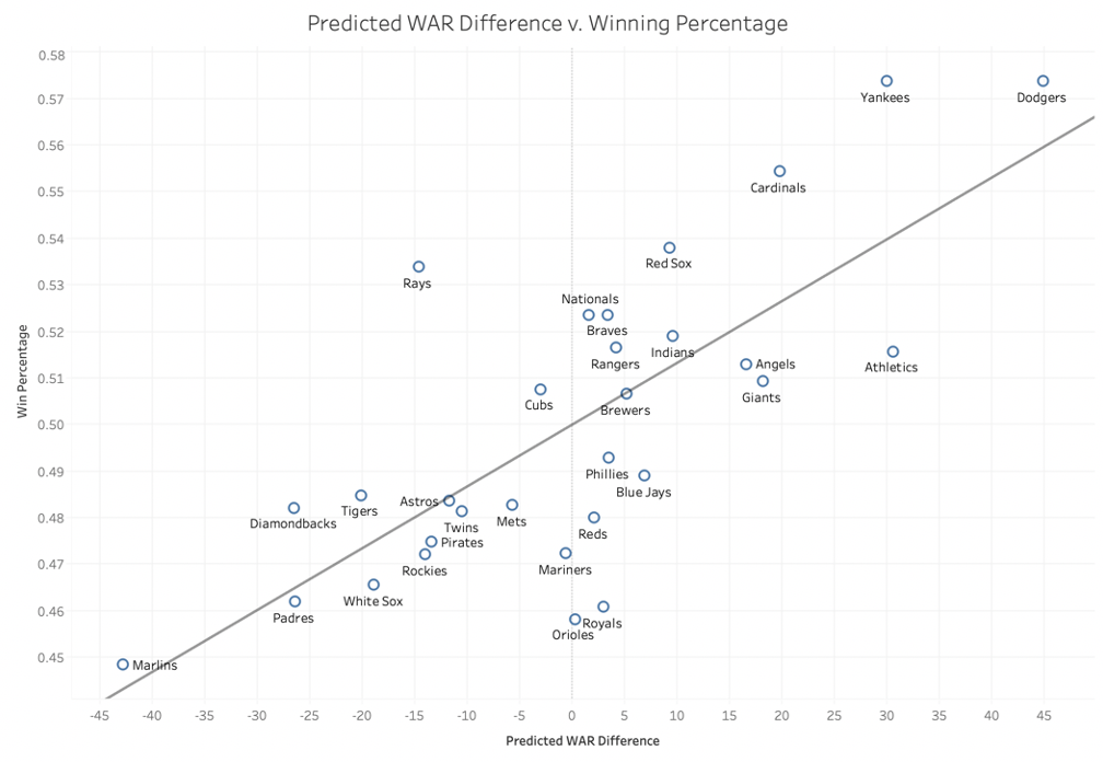
One of the more interesting things about the results of my research is the relationship between a team’s winning percentage and the difference between the WAR they were predicted to receive and the WAR they were predicted to trade away. As can be seen in the graph above, as a team’s predicted WAR difference increased, their winning percentage also increased. This validates for me that my models did a great job in assessing player’s trade values. As for which teams did the best overall, both in reality and according to my models, the Los Angeles Dodgers did the best with a predicted difference of 44.89 WAER and an actual difference of 31.1 WAR. As for the worst team, again both in reality and according to my models, it was the Miami Marlins with an actual difference of -31.1 and a predicted difference of -42.86.
Conclusions
I believe my research shows that teams that do well in trades generally do well on the field, as displayed by the graph above. Additionally, I feel that my models did an outstanding job at modeling teams’ success in trades. Based on important variables for each of three different player categories. The different categories for each position group represent an important characteristic for that particular group that MLB teams should always be considering. Finally, an extension of this project that I am definitely interested in is expanded my trade dataset to include prospects. Unfortunately, the metrics that I included were challenging to find for prospects, so I could only evaluate trades that involved major league players. Prospect evaluation is an extremely important aspect in baseball for teams, as prospects represent the future of the sport and teams are often just as concerned about their future as they are about their present. Therefore, prospects would be an interesting extension to this project. Overall, however, my research still answers my research questions and determines which teams are the best “traders” in baseball.