
By Alejandro Pesantez – Syracuse University ’21
Abstract
This research looks to analyze NFL player season stats during the 2009-2017 NFL seasons. The type of analysis that was done on this data was hierarchical clustering. This was done in order to cluster each offensive skill position (Quarterback, Running Back, and Wide Receiver), into different “cluster” groups, and to see which cluster for each positional group gives the best chance for a team to win. The data was collected from the nflscrapR GitHub which included passing, receiving, and rushing stats from the 2009-2017 NFL seasons. Some statistics that were used from each dataset were, passing yards, rushing yards, receiving yards, and other basic football statistics for the positions were used.
Introduction
Using clustering techniques in sports has been trending a lot recently. It’s been used in basketball, soccer, and many other sports, however, football has barely even touched the surface of using clustering techniques to analyse data. Since this is the case, I decided I wanted to cluster quarterbacks, running backs and wide receivers separately to see which type of player for each offensive skilled position gives a team the best chance to win.
In order to do this, I chose to use the clustering technique of hierarchical clustering. Once each position group has been clustered, the clusters are then compared to their perspective WPA (win probability added) to see which group of players are best for winning at each offensive skill position.
These clusters are then compared to the average actual winning percentage of each cluster during the 2009-2017 NFL seasons to see if history proves that the “best” cluster for each position found in this analysis is truly the best.
Method
The clustering technique used for this research is hierarchical clustering. With hierarchical clustering, initially each data point is considered an individual cluster. At each iteration, the similar clusters merge into other clusters until one or K clusters are formed. In order to find the optimal amount of “K” clusters I used the elbow and silhouette method for each position group.
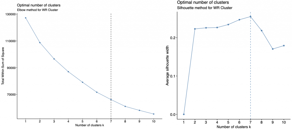
Once the optimal number of clusters were decided for the Quarterback, Wide Receiver, and Running Back data (4, 5, and 7 clusters respectively), the hierarchical clustering on the data was ran. The final dataset for the Wide Receiver data contained 3,264 observation with 43 variables, the Quarterback dataset contained 1,355 observation with 41 variables, and the Running Back dataset contained 2,168 variables with 49 variables.
Results
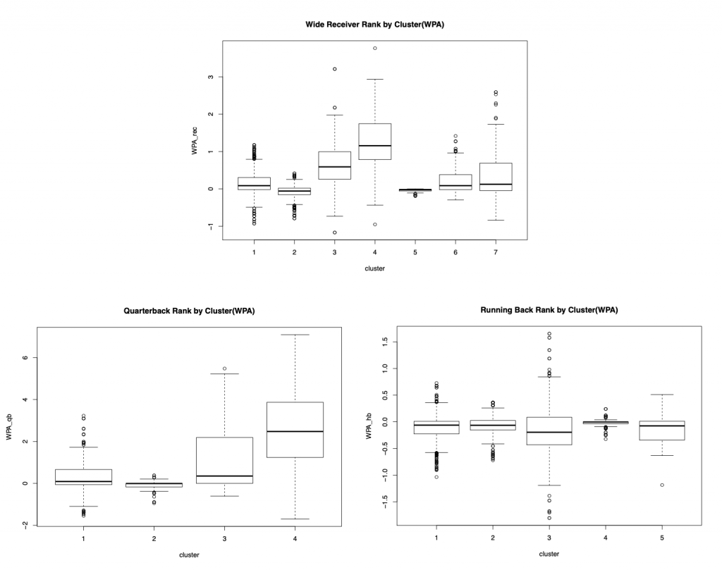
Once the clusters were done and looked at compared with WPA for each position, the clusters were then compared to the actual win percentage of the clusters from the 2009-2017 season. This was done by averaging each player’s win percentage in each cluster.
The results were similar when compared to the results of the clusters that looked at WPA. The distributions of the clusters almost look identical when looking at the bar charts and boxplots. Cluster 4 again is the best cluster in each position group in terms of winning for both the analyses that were done.

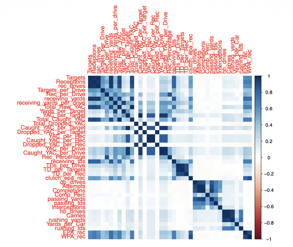
The final observation made from this research shows what statistics the best clusters are good at or not good at for each position group. The statistics I chose to look at were statistics that correlated the best with the WPA for each position group. There are also statistics that people would be interested in knowing given the position of a given cluster.

Conclusions
In conclusion, clustering NFL player season data from 2009-2017 , really shows what possibilities could come from clustering data from the NFL. Due to the fact of there not being much publicly available data about the NFL it is hard to get more in depth about clustering positions. I would love to work on this further to have the height, weight, age, and even combine statistics for these players, which I think would make this type of analysis a lot more interesting.
The only feasible conclusions that I can make about my results as of now, is that the players in each of the “best” clusters I found are the type of players you want on your team. In the Wide Receiver cluster, there were players such as 2012 Calvin Johnson, 2015 Julio Jones, and 2015 Odell Beckham Jr. In the Quarterback cluster, there were players such as 2011 Tom Brady, 2013 Peyton Manning, and 2011 Drew Brees. In the Running Back cluster, I had players such as 2011 Chris Ivory, 2013 C.J Anderson, and 2017 James Conner.
The only other conclusion about the results that could be made is that Running Backs could truly be not as valuable as they once were in the past, since the cluster distributions when looking at winning percentage and WPA are relatively the same or very similar across each cluster, inferring that it doesn’t matter what type of running back you have.
References
- 2017 NFL Standings & Team Stats. Pro. (n.d.). https://www.pro-football- reference.com/years/2017/index.htm.
- NBA Lineup Analysis on Clustered Player Tendencies: A new approach to the positions of basketball & modeling lineup efficiency. MIT Sloan Sports Analytics Conference. (n.d.). https://www.sloansportsconference.com/research- papers/nba-lineup-analysis-on-clustered-player- tendencies-a-new-approach-to-the-positions-of- basketball-modeling-lineup-efficiency.
- Patlolla, C. R. (2020, May 29). Understanding the concept of Hierarchical clustering Technique. Medium. https://towardsdatascience.com/understanding-the- concept-of-hierarchical-clustering-technique- c6e8243758ec.
- Ryurko. (n.d.). ryurko/nflscrapR-data. GitHub. https://github.com/ryurko/nflscrapR-data.
Acknowledgements
I would like to thank Dr. Rodney Paul, who has helped guide me through the research process. I would also like to thank my fellow classmate Jonathan Bosch for helping me think of this idea. And lastly, I would like to thank Ron Yurko for putting together the nflscrapR package which makes it very easy to get NFL statistics.