
By Fletcher Wilson – Syracuse University ’20
Background
Similar to the unique structuring of each of the four major sport leagues, the TV rights of each league also find themselves distinctly structured. Different leagues share revenue differently, as a result, each league tailors its TV contract to be most beneficial for their system revenue sharing. With each step further into the digital age, and every year an old contract expires, league execs and cable company execs look to push the envelope with new ideas and propositions to maximize their wealth. Consequently, the past decade was full of new and groundbreaking deals, unlike the simple contracts of old.
At its core, much about the NBA remains different than the MLB: their target audiences, game speed, and type of athletes, to name a few, yet both have their all-time legends. The primary difference between an NBA star and an MLB star is the significant impact on both attendance and cable TV ratings an NBA star will have. In a 1997 study about the effect of superstars, using M. Jordan, L. Bird, E. Johnson, I. Thomas, and Shaquille O’Neal, Bernd Frick found that superstars largely impact road attendance, and when it came to cable tv ratings there was a positive effect of the presence of a super star playing for the home or visiting team. The NBA remains a league driven by talent and star power, yet Frick concludes with the statement that a team’s overall productivity was always more important than star power. Frick also conducted a relevant study in the Bundesliga, where he looked at the effects of superstars compared with that of local heroes(MVP of team with no superstars), and found the two had similar effects. This brings about a question of whether superstars or fan favorites put more people in seats. It also becomes relevant to look into what factors driving NBA, NFL, or MLB ratings can be transferred and applied to other sports. Further investigation into these findings across more sports could reveal valuable new information.
Data
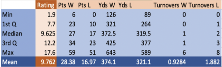
Data collection proved the most challenging yet critical aspect of the work, and as per usual, all the best data either cost money or was inaccessible without the right credentials. After several attempts to suede the kind yet stingy people of Nielsen to offer up their data to no avail, it became evident the source of the data would have to come from publicly available ratings data and attendance numbers. Due to the unique structuring of each league’s schedule and television contacts, certain ratings and attendance numbers were available on a seasonal or weekly basis. To best understand the factors driving ratings and attendance, we quantify and incorporate several similar aspects across each league. In addition to better grasp the uniqueness of each situation, first we must look to the individual data collection for each sport and then to a month during which all sports saw competition. Included are summaries for variables used in modeling. Through use of a series of dummy variables, the NFL data set now included whether the game featured the defensive or offensive rookie of the year, current years or reigning MVP, as well as that season’s defensive player of the year or passing, rushing, and receiving leaders. The inclusion of these allows for a measure of an individual players impact on the ratings; furthermore, it encompasses nearly all aspects of the game, save special teams.
In the NBA, we turn to dummy variables regarding league leaders in various statistical categories as well as the winners of the NBA’s various awards. Including within this category both awards (most valuable player, defensive player of the year, rookie of the year, and six man of the year) and statistical leaders(points, rebounds, assists, steals, three points, and blocks) measures the influence of popular stars and quality basketball players alike. Similarly, it allows for the creation of parallels to other leagues, making it easier to identify similar factors driving viewership.
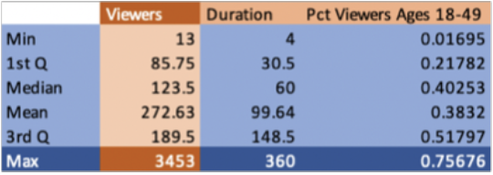
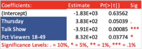
The October sport data set provides insight to the summaries of the ratings and percent of viewers 18-49 for each sports network. Each channel offered several different programs including live coverage as well as re-airings of games, talk shows, and pre/post game coverage. Measuring these variables, critical to understanding which leagues succeed in what aspects, requires the use of dummy variables again. Differentiating between live airings, re-runs, talk shows, and post-game shows offer further insight to each leagues successes and short comings in the development of their media empires.
| Golf Channel | MLB Network | NFL Network | NBA TV | |
| Age % Viewers 18-49 | 18.28% | 26.80% | 48.58% | 58.16% |
Methodology
Multicollinearity
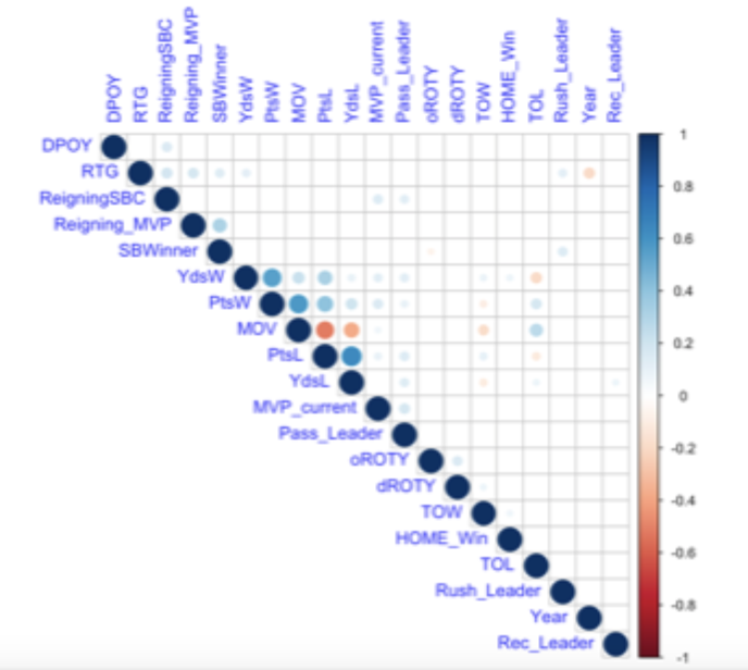
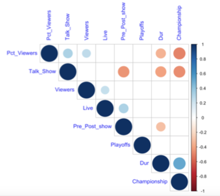
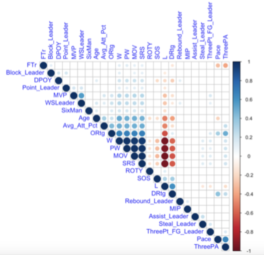
Initially it appeared multicollinearity could cause problems in the data with the multitude of player attributes and statistics included. Often statistics find themselves derived from other stats, and similarly it is not uncommon for Most Valuable Players to play for championship winning teams. The creation of a correlation chart featuring all variables in each model works to ensure a thorough sample. To better visualize this, we create respective correlation matrices featuring the variables of each model, then extract the correlation coefficients and p-values for each. This provides us with a correlogram, essentially a chart outlining the different positive and negative correlations of the variables, as well as correlation coefficients. Adding color, we display positive correlations in blue and negative correlations in red. Located to the right of the correlograms, note the color legend, indicating the color intensity proportional to the correlation coefficient.
Linear Regression
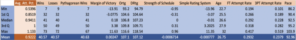
With the orientation of the data and desired outcome, a linear model came forth as the most logical choice. Each data set receives unique modeling, while similar dependent and independent variables are tested. In the linear model for NFL TV ratings, the dependent variable is of course rating. Included as independent variables we see points, yards, and turn overs of both the winning and losing team. Dummy variables include a home team win, and whether the game featured the: reigning MVP, current MVP, Offensive Rookie of the Year, Defensive Rookie of the Year, Defensive player of the Year, Rushing Leader, Passing Leader, Receiving Leader, Reigning Super Bowl Champion and that year’s Super Bowl Champion. Lastly, we identify the home, away, and underdog teams, along with the underdog’s spread and the year. Using average attendance as the dependent variable in the NBA model, we next include Pythagorean wins, losses, margin of victor, season average offensive rating, season average defensive rating, simple rating system, team average age, free throw rate, three point attempts, pace, division, and team. To account for Six Man of the Year, MVP, Defensive Player of the Year, and Rookie of the Year, along with the season leaders in the following categories: points, rebounds, assists, steals, three points, blocks, and win shares. The final linear regression revolving around ratings in October features rating as the dependent with less independent variables. Independent variables include the sport, day, date, duration, and the percentage of viewers ages 18 to 49, with dummy variables for whether or not the program was live, a talk show, pre/post game show, championship game, or playoff game. Positive and significant relationships between variables within these models should signify the variable increases viewership or attendance, while negative significant relationships signifies the variable will likely decrease said factors. Each linear regression effectively models the influence of the respective independent variables on ratings and attendance.
Results and Conclusion
Through the use of linear modeling, we find the results of each pointing to the significance of captivating and telling variables. In some cases, similar variables hold similar relationships across sports, yet in other cases they appear as non- factors. Included below are the significant variables found in each regression.
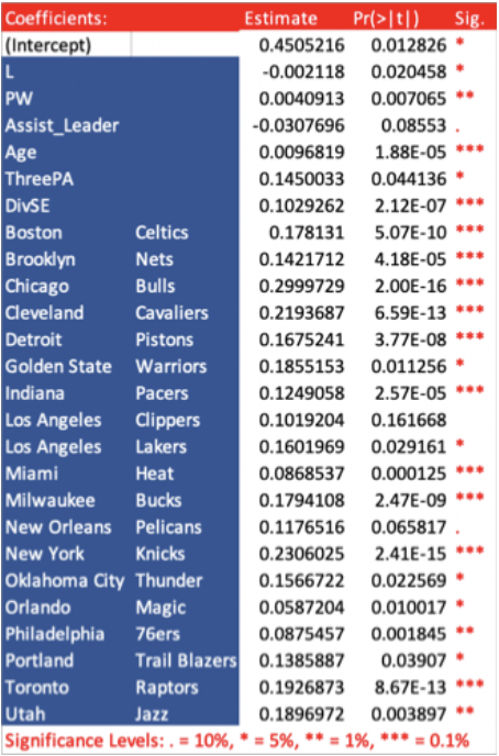
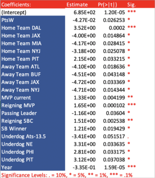
Within the linear model for NBA attendance lay various eye opening, positively correlated, and significant variables. The positive correlation between age and average attendance percentage instantly incepts a cornucopia of explanations for the relationship. Bad teams in the midst of a rebuild may feature more rookies or young talent. Conversely, fans across the NBA may wish to attend games featuring players they already know and have watched for longer, leading to an older average age team seeing higher average attendance. The TV Ratings across the NFL linear model presents its own significant variables, many at different degrees of positive and negative correlation(seen in [Figure 8]). Over the past 5 years we look to teams with significant and negative correlation to ratings, including home and away teams. When at home, the Miami Dolphins, New York Jets, and Jacksonville Jaguars see lower ratings. The Jets and Dolphins play in the same division, along with the New England Patriots and Buffalo Bills, which the Patriots have reigned over the past two decades. From this we surmise that home fans have likely grown weary of watching their bad teams play bad competition or lose to the Patriots. Next, the effect of winning the previous Super Bowl appears stronger than the effect of going on to win the Super Bowl. Making the scheduling for next year’s season after knowing the Super Bowl winner may explain some of the correlation here, as teams that won receive more nationally televised and prime time games. , we identify similar trends in the reigning MVP as opposed to the player who would go on to win MVP. Again, fans trend towards watching a player they know has MVP caliber, not an elite player that would go on to win MVP. Captivating results indeed.
References
[1] Dyer, Kristian. “Baseball Attendance Drops at MLB Stadiums for Fifth Straight Year.” Fox Business, Fox Business, 20 Sept. 2019, https://www.foxbusiness.com/features/on-declining-mlb-attendance-former-executive- says-substantive-changes-must-be-made.
[2] Edwards, Craig. “Estimated TV Revenues for All 30 MLB Teams.” FanGraphs Baseball, 25 Apr. 2016, blogs.fangraphs.com/estimated-tv-revenues-for-all-30-mlb-teams/.
[3] Edwards, Craig. “Those Disastrous World Series TV Ratings.” FanGraphs Baseball, 30 Oct. 2018, https://blogs.fangraphs.com/those-disastrous-world-series-tv-ratings/.
[4] Frick, Bernd, editor. BREAKING THE ICE: the Economics of Hockey. SPRINGER, 2018.
[5] Graziano, Dan. “NFL CBA Approved: What Players Get in New Deal, How Expanded Playoffs and Schedule Will Work.” ESPN, ESPN Internet Ventures, 15 Mar. 2020, www.espn.com/nfl/story/_/id/28901832/nfl-cba- approved-players-get-new-deal-how-expanded-playoffs-schedule-work.
[6] Humphreys, Brad R., and Candon Johnson. “The Effect of Superstar Players on Game Attendance: Evidence from the NBA.” SSRN Electronic Journal, 31 July 2017, doi:10.2139/ssrn.3004137.
[7] Kaplan, Daniel. “NFL’s TV Deals Hedge against Work Stoppage.” Sports Business Daily, 29 Oct. 2018, www.sportsbusinessdaily.com/Journal/Issues/2018/10/29/Leagues-and-Governing-Bodies/NFL-TV-deals.aspx.
[8] Lucia, Joe, et al. “MLB Local Viewership down 4% in First Half, Led by Drops from Large Market Teams.” Awful Announcing, 22 July 2019, https://awfulannouncing.com/mlb/mlb-local-viewership-down-4-in-first-half-led-by-drops-from-large-market-teams.html.
[9] Moran, Ed. “Another Year Of Declining Attendance: How Worried Should MLB Be?” Front Office Sports, 7 Oct. 2019, https://www.frntofficesport.com/mlb-attendance-2019-2/.
[10] “NFL Blackout Rule: Richard Nixon Hated It.” The Denver Post, St. Paul Pioneer Press, 29 Apr. 2016, www.denverpost.com/2013/07/07/nfl-blackout-rule-richard-nixon-hated-it/.
[11] Ourand, John. “A Ratings Home Run: Machado, Harper Drive Increases in Local Viewership.” Sports Business Daily, 22 July 2019, https://www.sportsbusinessdaily.com/Journal/Issues/2019/07/22/Research-and-Ratings/MLB- RSNs.aspx.
[12] Thurm, Wendy. “Dodgers Could Be Last Team To Strike Gold With Local TV Deal.” FanGraphs Baseball, 26 July 2013, blogs.fangraphs.com/dodgers-could-be-last-team-to-strike-gold-with-local-tv-deal/.
[13] Woo, Marcus. “Resting Healthy NBA Players During the Season May Not Help Them in Playoffs.” Inside Science, 18 Oct. 2017, https://www.insidescience.org/news/resting-healthy-nba-players-during-season-may-not-help-them- playoffs.